A Survey of Model-Based Reinforcement Learning

Abstract

In recent years, development in Reinforcement Learning (RL) contributes to super-human performances in games, such as Go, Chess, and StarCraft, as well as in daily contexts, including conversation and robot control. However, RL learns through trial-and-error, which potentially requires a huge amount of data. A new line of research called model-based RL (MBRL) can largely alleviate the data requirement both empirically and theoretically. This survey reviews the recent advances in MBRL mainly from two perspectives, i.e., how to obtain a model and how to obtain a policy, whereas the latter topic can be further divided into learning-free and learning-based sections. The survey ends with a brief discussion of future directions.

Introduction

Reinforcement Learning

In recent years, development in Reinforcement Learning (RL) contributes to super-human performances in games, such as Go[^silver2016mastering], Chess, and StarCraft, as well as in daily contexts, including conversation and robot control. Especially, large language models combined with RL with Human Feedback (RLHF) show great potential in aligning with human intentions and are in some ways shaping the world we live in.

Despite its great influence, RL itself seems straightforward. The goal of RL is to find a policy that maximizes the sum of future rewards. Formally, a Markovian Decision Process (MDP) is denoted as $\langle S, A, P, R, \gamma \rangle$, where $S$ denotes the state, $A$ the action, $P$ the transition probability, $R$ the reward, and $\gamma$ the discount factor. At each state $s_t$, the agent takes an action $a_t$ and observes the next state $s_{t+1}=f(s_t, a_t)$ as well as a reward $r_t$. The goal is to maximize future rewards: $G_t = \sum_i \gamma^i r_{t+i}$.

Model-Based Reinforcement Learning

However, common model-free RL algorithms learn purely from trial-and-error, which requires large amounts of data and direct interaction with the world (low sample efficiency).

To address the sample efficiency problem, we turn to Model-Based RL (MBRL) for solutions, whose core framework is:

while not converged:
    1. Collect data D under the current policy Π
    2. Learn a model M with the collected data
    3. Improve the policy Π using the model M

Most MBRL algorithms divide the problem into two separate processes, one is to learn a world model that can represent the transition dynamics and sometimes the reward dynamics, and the other is to learn a policy that can be either a learning-based, parameterized network or a planning or searching process. The main design points of MBRL can thus be defined as model learning and model usage.

Paper Organization

We will begin with model learning. These methods vary a lot, from the simplest model that only predicts one-step transition, to the most complex model that builds upon modern structures such as transformers.

Then, we will dive into the topic of model usage. In MBRL, the policy can either be learning-free or learning-based. In this survey, we will present three types of learning-free policies, namely, random shooting, Monte-Carlo tree search, and linear quadratic regulator. Next, we will turn to learning-based policies where the policy is parameterized by a neural network. There are various learning processes, and we will mainly focused on direct gradient, MFRL, and imitation learning cases.

We will end the survey with a brief discussion of future directions.

Model Learning

The most important process in MBRL is model learning. An ideal model should give accurate prediction of the future situation and potentially tackles the problem of high-dimensional, multi-modal, complex observation input.

Transition Model

The most straight-forward method would be to directly model the one-step transition function $s_t=f(s_t,a_t)$. Using neural network to approximate the function, we can thus use supervised learning to minimize the mean-squared error between predicted states and real states. To avoid the distribution mismatch, we constantly rollout the current policy to add on-policy trajectories into the training dataset. To alleviate the model compounding errors, we normally apply Model Predictive Control (MPC), executing only the first action in the predicted action series and discarding the subsequent actions. In other word, we replan every step to maintain a relatively on-policy planning. This gives us the general training framework of dymacis model as illustrated:

1. Run policy $\Pi(a_t \mid s_t)$ to collect dataset D = {(s, a, s')}
2. while not converged:
    a. Train the dynamics model f(s, a) on dataset D (minimize loss)
    b. Rollout policy via f(s, a) to plan actions
    c. Execute first planned action, observe resulting s'
    d. Add (s, a, s') to D

Early algorithms apply this line of training and obtain satisfying results. For example, in Mb-Mf, the authors uses such direct training and obtain comparable results to model-free RL with less samples in low-dimensional cases.

Model Uncertainty

However, using a single transition model is often insufficient due to overfitting and model bias. Overfitting problems are common in supervised learning, which means that the neural network performs well on training data but poorly on test data. With MBRL, a new challege called “model bias” arises, in that policy optimization will exploit regions where the model is not sufficiently trained and leads to catastrophic failures. Consider the following example. An agent is trying to reach the edge of a cliff. The closer the agent is to the cliff, the less data is available to train the dynamics model, and therefore the less accurate the model is. Thus, if the agent relies solely on the model to plan its actions, it will fall off from the cliff constantly.

This problem can be alleviated if we can express the model uncertainty in some way. When the agent is aware of its deficiency, it can perform less aggressive policy optimization to avoid exploiting the areas that the model is uncertain about. In the previous example, if the agent knows that it is uncertain around the cliff, then it can be more cautious and take smaller steps as it reaches closer to the cliff. Note that, different from the aleatoric or statistical uncertainty induced by the noise in the dataset, this model uncertainty is epistemic, resulting from model-overfitting and insufficient training.

Another popular fix is to train an ensemble of models and evaluate their consistency. The similarity of the results given by different models can represent the model certainty. The more similar the results, the more accurate the prediction is, and therefore the more aggressive the policy can be.

ME-TRPO replaces the single dynamics model with an ensemble of dynamics models and uses TRPO to capture the model uncertainty and update its policy accordingly. SLBO replaces the model learning objective in ME-TRPO of a multi-step prediction \(L(s_{t:t+h},a_{t:t+h})=\frac{1}{H}\Sigma_H||(\hat{s}_{t+i}-\hat{s}_{t+i-1})-(s_{t+i}-s_{t+i-1})||_2\). This strengthens the model’s abality of making long-term predictions.

Inspired by meta-policy training, MB-MPO tries to learn an adaptive policy that can quickly adapts to any of the models in the learned ensemble. As in typical meta-RL settings, the algorithm is divided into two parts, where the first one trains a general policy, and the second one performs a few policy updates to adapt the general policy into a specific environment (in this case, the environment given by a dynamics model). In MB-MPO, the general policy is trained via TRPO as in ME-TRPO, and the adaptive polices are trained with vanilla policy gradient. The potential benefit is that the policy is robust enough to ignore the model errors and can quickly adapt to real world scenarios.

While the above works use the dynamics model to generate full trajectories, MBPO only uses the dynamics model to augment existing data. Instead of training a policy inside of the learned model, it uses real world data with short model rollouts to improve its policy with off-policy model-free RL. In this way, MBPO avoids long-term prediction of the model and thus allievates the compounding model error.

A recent work, however, proves that the model ensemble approach is valid only because it regularizes the Lipschitz condition of the value function through the generated samples. Therefore, MBRL algorithms with a single dynamics model and a regularized value function can outperform those with an ensemble of dynamics models.

Variational Auto-Encoder and Latent Models

To deal with high-dimensional inputs and partially observable environments, we can use variational auto-encoder models to extract the features of the states and express them in a simple latent space. The learned approximate posterior, also called encoder, can take in various forms, from the single-step encoder $q_\Phi(s_t \mid o_t)$ to the full smoothing posterior $q_\Phi(s_t, s_{t+1} \mid o_{1:T},a_{1:T})$. Empirically, the simplest encoder is sufficient.

Assume we have a deterministic encoder with the form $q_\Phi(s_t \mid o_t)$ that presents states as $s_t=g_\Phi(o_t)$, the loss of the world model can be expressed as follows, where the three terms correspond to latent space dynamics, image reconstruction, and reward model, respectively. \(\max_{\Phi,\Theta} \frac{1}{N}\Sigma_N\Sigma_T\log p_\Theta(g_\Phi(o_{t+1,i}) \mid g_\Phi(o_{t,i}),a_{t,i})+\log p_\Theta(o_{t,i} \mid g_\Phi(o_{t,i}))+\log p_\Theta (r_{t,i} \mid g_\Phi(o_{t,i}))\)

Recent works often employ this approach. In VPN, the encoder is $f_\theta^{enc}(s_t \mid o_t)$, and the transition model is $f_\theta^{trans}(s_{t+1} \mid o_t,s_t)$. From the abstract state, the model has to predict the immediate reward and discount from $f_\theta^{out}(r_t,\gamma_t \mid o_t,s_t)$, and the value of the next abstract-state from $f_\theta^{value}(V_\theta(s_t) \mid s_t)$. With these models representative of the entire world, VPN uses a modified depth-first search algorithm to plan the optimal path. Other examples include SOLAR, MuZero, etc.

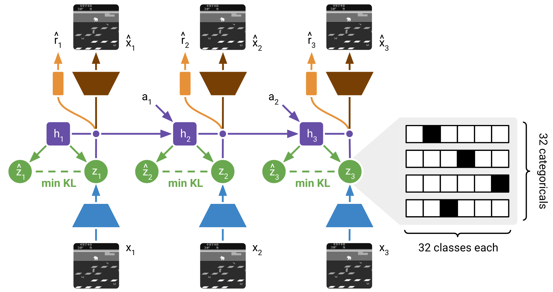
PlaNet improves the performance of the latent model via Recurrent State Space Model (RSSM). The state in RSSM is a combination of a hidden state $h_t$ and a posterior state $z_t$, where the former captures the time sequence with RNN, and the latter encodes the high-dimensional input into a latent representation. The RSSM thus consists of six parts: a recurrent model that generates the hidden states $h_t=f_\phi(h_{t-1},z_{t-1},a_{t-1})$, a representation model that encodes the observation and the hidden state into a posterior state $z_t \sim q_\phi(z_t \mid h_t,o_t)$, a transition model that predicts an approximate prior state based purely on hidden states \(\hat{z}_t\sim p_\phi(\hat{z}_t \mid h_t)\), an image predictor that reconstruct the input observation \(\hat{o}_t\sim p_\phi(\hat{o}_t \mid h_t,z_t)\), a reward predictor that predicts the reward \(\hat{r}_t\sim p_\phi(\hat{r}_t \mid h_t,z_t)\), and a discount predictor that predicts the discount (i.e., whether the episode ends) \(\hat{\gamma}_t\sim p_\phi(\hat{\gamma}_t \mid h_t,z_t)\). Later in Dreamer series, the latent space is further discretized to better present latent-space computations.

Recently, a surge of research tries to employ modern architectures to the model. This includes TAP, which learns low-dimensional latent action codes with a state-conditional VQ-VAE, and TWM that utilizes the Transformer-XL architecture to learn long-term dependencies while staying computationally efficient.

Planning and Searching

Given an accurate model, we can apply planning or searching algorithms as in typical control settings. Theoretically and empirically, this combination reaches super-human level results within a relative short period of training time. In this section, we will present three classic learning-free algorithms, namely, random shooting, Monte Carlo tree search, and linear quadratic relugator.

Random Shooting

Random shooting is a method that is easy to implement, straight-forward and works well within low-dimension, short-horizon settings. It randomly generates K action sequences and then calculates the cumulative rewards of each action series based on the learned dynamics. When interacting with the environment, the agent chooses the action series with the highest predicted reward. In Mb-Mf, the authors employ the Model Predictive Control (MPC) as introduced in Section \ref{sec:transition}.

To improve its performance, instead of randomly generating actions, the model selects actions that may result in higher rewards. A common approch is Cross Entropy Method (CEM) that iteratively fits a Gaussian distribution of the most promising actions and then samples from the distribution, as depicted in Algo\ref{alg:cem}. PETS, POPLIN, and PlaNet adopts such method. In POPLIN, the authors find that differently executed CEM can lead to different performance, and the best place to add the Gaussian noise is in the parameter space.

while in action optimization:
    1. Sample K candidate action sequences from distribution p(A)
    2. Evaluate predicted rewards for each
    3. Select top M elite sequences
    4. Update p(A) to fit elites
    5. Repeat until done

Monte Carlo Tree Search (MCTS)

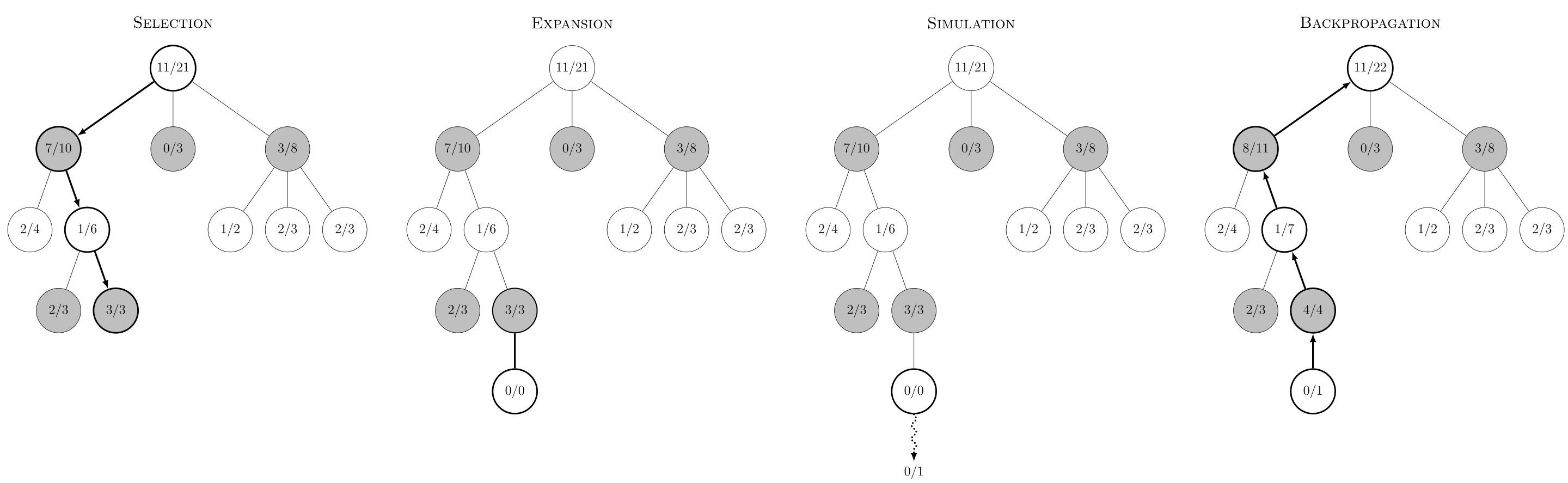
MCTS combines planning and search, and is crucial in AlphaGo, AlphaZero, and MuZero. It builds a tree that simulates many possible futures, balancing exploration and exploitation at each node. Policy networks, value networks, and learned models can all be combined via MCTS.

Linear Quadratic Regulator (LQR)

LQR comes from control theory. The agent minimizes a quadratic cost in state (x_t) and action (u_t), assuming linear-Gaussian dynamics:

• Backward recursion computes optimal gains with system matrices.
• Forward recursion rolls out the best actions using these gains.

Policy Learning

Model-based RL can also use parameterized policies learned by:

• Direct gradient (backpropagating rewards through the learned model). Gradient-based fine-tuning resembles the PILCO family and Dreamer.
• Model-free RL within a learned model environment—e.g., DYNA, q-learning, actor-critic, and actor-critic with ensembles.
• Imitation learning and distillation—using expert data or controllers as initial policy, or using ensembles for robust initialization.

Methods such as Dreamer, MBPO, SLBO, and others combine these approaches with model-based rollouts, direct gradient, or other hybridizations.

Conclusion

Sample efficiency in RL remains a major research target, and MBRL is an effective approach. MBRL research focuses on model learning (dynamics, uncertainty, latent space, transformers) and policy application (planning, searching, policy gradient, actor-critic, imitation). As hardware and model architectures advance, so too does the practical power of MBRL in control and AI planning.

References

• [1] Sutton, R. S., and Barto, A. G. (2018). Reinforcement Learning: An Introduction. 2nd Edition.
• [2] Nagabandi, A., Kahn, G., Fearing, R. S., and Levine, S. (2018). Neural Network Dynamics for Model-Based Deep Reinforcement Learning with Model-Free Fine-Tuning. ICRA.
• [3] Hafner, D., Lillicrap, T., Norouzi, M., and Ba, J. (2019). Dream to Control: Learning Behaviors by Latent Imagination. arXiv:1912.01603.
• [4] Silver, D., Hubert, T., Schrittwieser, J., Antonoglou, I., et al. (2018). A general reinforcement learning algorithm that masters chess, shogi, and Go through self-play. Science.
• [5] Janner, M., Fu, J., Zhang, M., and Levine, S. (2019). When to Trust Your Model: Model-Based Policy Optimization. NeurIPS.